Catherine Hood Consulting
Frequently Asked Questions Categories:
Definitions and Concepts FAQ
- What is a time series?
- What is seasonal adjustment?
- What kind of data do we need for seasonal adjustment?
- Why seasonally adjust data?
- How much data do I need to get a reasonable adjustment?
- What are the components of a time series decomposition?
- What effects are removed during seasonal adjustment?
- What is an ARIMA model?
- What is a regARIMA model?
- How do I generate a seasonally adjusted series?
- What are seasonal filters?
- What are trend filters?
- Why do the seasonal factors change when new data is added?
- How do I choose between additive and multiplicative models?
- What is an indirect (or a direct) adjustment? Why would I need one?
1. What is a time series?
A time series is a sequence of measures of a given phenomenon taken at regular time intervals such as hourly, daily, weekly, monthly, quarterly, annually, or every so many years.
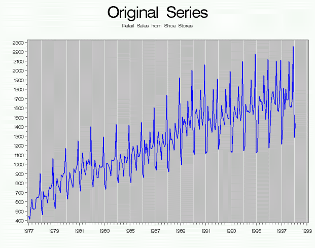
An example of a time series is shown below. This time series happens to be Retail Sales from Shoe Stores.
2. What is seasonal adjustment?
Seasonal adjustment is the process of estimating and removing the seasonal effects from a time series, and by seasonal, we mean an effect that happens at the same time and with the same magnitude and direction every year. The basic goal of seasonal adjustment is to decompose a time series into several different components including a seasonal component and an irregular component. Because the seasonal effects are an unwanted feature of the time series, seasonal adjustment can be thought of as focused noise reduction.
For more information on why seasonal effects are unwanted, please see the paper (in PDF) "Why Seasonal Adjustment" by James Ashley.
3. What kind of data do we need for seasonal adjustment?
We need a time series for seasonal adjustment. Because seasonal effects are annual effects, the data must be collected at a frequency less than annually, usually monthly or quarterly. For the data to be useful for time series analysis, the data should be comparable over time. That means
- the measurements should be taken over discrete (nonoverlapping) consecutive periods, i.e., every month or every quarter, and
- the definition of the concept and the way it is measured should be consistent over time.
4. Why seasonally adjust data?
Economists, policy makers, and consumers use time series we publish to make decisions. They try to identify important features of economic series such as direction, turning points, and consistency between other economic indicators. Sometimes seasonal movements can make these features difficult to see, so we publish economic series with the seasonal movements removed for those who prefer to view data without seasonal movements.
There is some information lost when a series is seasonally adjusted; therefore it is also useful for many people to have both the original series and the seasonally adjusted series available for analysis.
For more information, please see the paper (in PDF) "Why Seasonal Adjustment" by James Ashley.
5. How much data do I need to get a reasonable adjustment?
X-12-ARIMA and X-13ARIMA-SEATS will work with four years of data. To get good regARIMA models (see question 8 for more information on regARIMA models), it is better to have at least seven years of data. Studies have shown that TRAMO/SEATS works best with at least six years of data.
Keep in mind that longer series aren't necessarily better. If the series has changed the way the data is measured or defined, it might be better to cut off the early part of the series to keep the series as homogeneous as possible. The best way to decide if your series needs to be shortened is to investigate the data collection methods and the economic factors associated with your series and choose a length that gives you the most homogeneous series possible.
If you have less than four years of data, please see the paper (in PDF) "Seasonal Adjustment for Short Time Series in Excel" for an outline of the steps to compute a seasonal adjustment, with examples.
6. What are the components of a times series decomposition?
In seasonal adjustment, a time series is usually broken down into the following components:
Trend or Trend-Cycle (T or C):
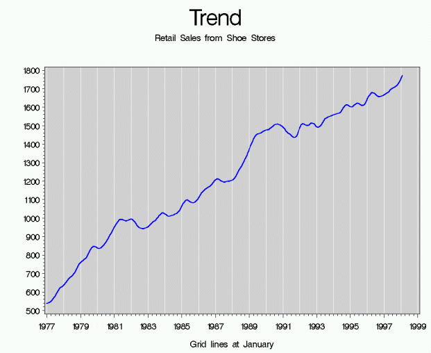
An estimate of the local level of the series derived from the surrounding recent (a year or two) observations. The trend is generally fairly smooth and includes movements and cycles longer than a year.
An example trend from Retail Sales from Shoe Stores.
Seasonal Effects (S):
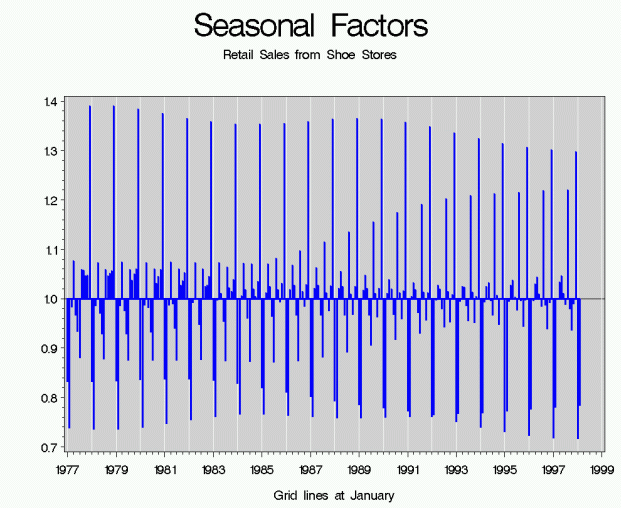
Effects that are reasonably stable in terms of annual timing, direction, and magnitude. Possible causes include natural factors (the weather), administrative measures (starting and ending dates of the school year), and social/cultural/religious traditions (fixed holidays such as Christmas).
An example of seasonal factors from Retail Sales from Shoe Stores.
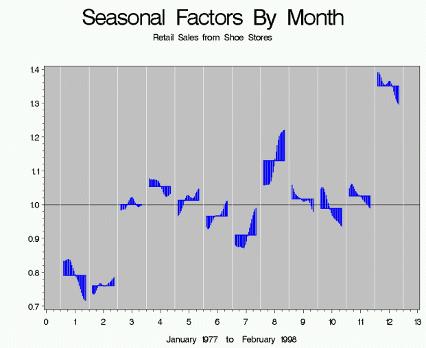
We can also look at the seasonal factors by month (again from Retail Sales from Shoe Stores).
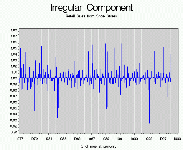
Irregular Component (I):
Anything not included in the trend-cycle or the seasonal effects (or in estimated trading day or holiday effects). Its values are unpredictable in regards to timing, impact, and duration. It can arise from sampling error, non-sampling error, unseasonable weather, natural disasters, strikes, etc.
An example irregular component from Retail Sales from Shoe Stores.
Trading Day Effects (TD):
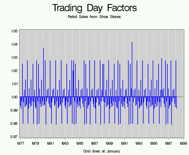
Recurring effects associated with individual days of the week. This occurs because only non-leap-year Februaries have four of each type of day - four Mondays, four Tuesdays, etc. All other months have an excess of some types of days. If an activity is higher on some days compared to others, then the series can have a trading day effect. For example, building permit offices are usually closed on Saturday and Sunday. Thus, the number of building permits issued in a given month is likely to be higher if the month contains a surplus of weekdays and lower if the month contains a surplus of weekend days.
An example of trading day factors from Retail Sales from Shoe Stores. Please note that the scale for the trading day factors is smaller than the scale of the seasonal factors.
Moving Holiday Effects (H):
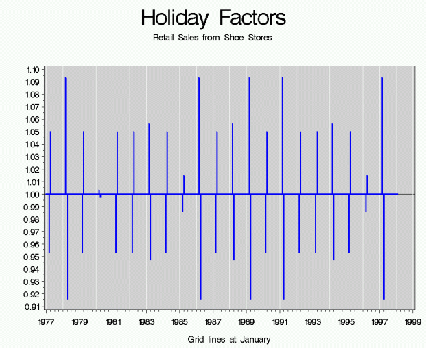
Effects from holidays that are not always on the same day of a month, such as Labor Day or Thanksgiving. The most important moving holiday in the US is Easter, not only because it moves between days, but can also move between months since it can occur in March or April.
An example of holiday factors from Retail Sales from Shoe Stores. For this particular series, the only holiday estimated is an Easter effect. Again, note that the size of the Easter effect is smaller than the size of the seasonal effect.
Combined Effects (S'):
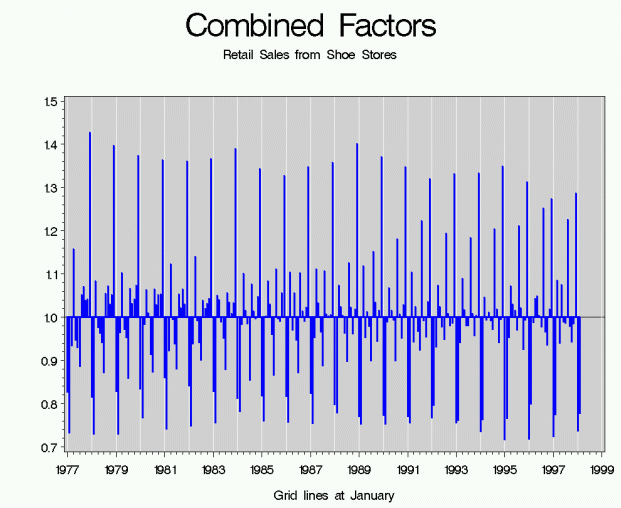
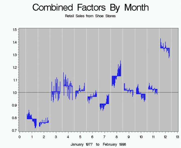
Since trading day and moving holiday effects are persistent, predictable calendar-related effects, we also want to remove these calendar effects from the seasonally adjusted series. The combined factors are the seasonal factors combined with the trading day and holiday factors.
An example of combined factors from Retail Sales from Shoe Stores.
We can also look at the combined factors by month (again from Retail Sales from Shoe Stores).
7. What effects are removed during seasonal adjustment?
During seasonal adjustment, we remove seasonal effects from the original series. If present, we also remove trading day and moving holiday effects. The seasonally adjusted series is therefore a combination of the trend and irregular components. (See question 6 above for definitions of these components.)
One common misconception is that seasonal adjustment will also hide any outliers present. This is not the case. If there is some kind of unusual event, we need that information for analysis, and outliers are included in the seasonally adjusted series.
8. What is an ARIMA model?
ARIMA (which stands for Auto-Regressive Integrated Moving Average) models are a group of models for describing the relationships between points in a time series and using that relationship to forecast the series. The auto-regressive part of the model uses past values (called lagged values) of the series to model the current value. Integrated refers to taking differences between lagged values. The moving average part of the ARIMA model uses lagged forecast errors. Note that this use of the phrase "moving averages" is not the same as when we talk about "moving averages" used in X-11-type seasonal filters (as discussed in question 12 below).
A seasonal ARIMA model would be designed as ARIMA(p,d,q)(P,D,Q) where
- p is the number of nonseasonal autoregressive terms,
- d is the number of nonseasonal differences,
- q is the number of nonseasonal moving average terms,
- P is the number of seasonal autoregressive terms,
- D is the number of seasonal differences, and
- Q is the number of seasonal moving average terms.
9. What is a regARIMA model?
A regARIMA model is a regression model with ARIMA errors. When we use regression models to estimate some of the components in a time series, the errors from the regression model are correlated, so we use ARIMA models to model the correlation in the errors.
Besides using regARIMA models to estimate regression effects (such as outliers, trading day, and moving holidays), we also use regARIMA models to forecast the series. Research has shown that using forecasted values gives smaller revisions at the end of the series.
10. How do I generate a seasonally adjusted series?
When generating seasonally adjusted series, it is important to use software specifically designed for the purpose of seasonal adjustment. Seasonal adjustment is more complicated than it might seem on the surface. For most series, seasonal adjustment can NOT be done properly by hand or with a spreadsheet program like Excel.
A good seasonal adjustment program has at least the following features:
- unbiased
- robust against outliers
- moving holiday and working/trading day estimation
- diagnostics
Seasonal adjustment is usually done with an off-the-shelf program. The three most popular programs are X-12-ARIMA and X-13ARIMA-SEATS from the U.S. Census Bureau and TRAMO/SEATS from Banco de Espana (Bank of Spain). The newest program from the U.S. Census Bureau is X-13ARIMA-SEATS which combines all the features of X-12-ARIMA with ARIMA-model-based adjustments from an implementation of the SEATS seasonal adjustment program.
X-13ARIMA-SEATS is used at the U.S. Census Bureau for all official seasonal adjustments in the publications, using options similar to those found in X-12-ARIMA. For more information on X-12-ARIMA and X-13ARIMA-SEATS, please see the questions in the FAQ related to X-12 and X-13. TRAMO/SEATS is used by some statistical offices and banks, primarily in Europe. For more information on TRAMO/SEATS, please see the questions in the FAQ related to TRAMO/SEATS.
11. What are seasonal filters?
A filter is a weighted average where the weights sum to 1. Seasonal filters are the filters used to estimate the seasonal component. Ideally, seasonal filters are computed using values from the same month or quarter, for example, an estimate for January would come from a weighted average of the surrounding Januaries.
The seasonal filters available in X-12/X-13 consist of seasonal moving averages of consecutive values within a given month or quarter. An n x m moving average is an m-term simple average taken over n consecutive sequential spans.
An example of a 3x3 filter for January 2003 (or Quarter 1, 2003) is:
2001.1 + 2002.1 + 2003.1 +
         2002.1 + 2003.1 + 2004.1 +
                  2003.1 + 2004.1 + 2005.1
___________________________________________
                    9
An example of a 3x5 filter for January 2003 (or Quarter 1, 2003) is:
2000.1 + 2001.1 + 2002.1 + 2003.1 + 2004.1 +
         2001.1 + 2002.1 + 2003.1 + 2004.1 + 2005.1 +
                  2002.1 + 2003.1 + 2004.1 + 2005.1 + 2006.1
_____________________________________________________________
                             15
12. What are trend filters?
Trend filters are weighted averages of consecutive months or quarters used to estimate the trend component.An example of a 2x4 filter for First Quarter 2005:
2004.3 + 2004.4 + 2005.1 + 2005.2 +
         2004.4 + 2005.1 + 2005.2 + 2005.3
___________________________________________
                    8
Notice that we are using the closest points, not just the closest points within the First Quarter like with the seasonal filters above. Notice also that every quarter has a weight of 1/4, though the Third Quarter uses values in both 2004 and 2005.
13. Why do the seasonal factors change when new data are added?
Keep in mind that the data used in the seasonal and the trend filters can go back several years.
Let's look at an example using X-12/X-13's seasonal moving average filters. For example, if the last point in your series is January 2013, and you're using 3x5 seasonal filters, the value at January 2013 will effect the estimates for Januaries in 2010, 2011, and 2012. You can see the value for January 2010 in the equations below.
The 3x5 filter for January 2010:
2007.1+2008.1+2009.1+2010.1+2011.1
       2008.1+2009.1+2010.1+2011.1+2012.1
              2009.1+2010.1+2011.1+2012.1+2013.1
________________________________________________
                      15
The 3x5 filter for January 2011:
2008.1+2009.1+2010.1+2011.1+2012.1
       2009.1+2010.1+2011.1+2012.1+2013.1
              2010.1+2011.1+2012.1+2013.1+2014.1
________________________________________________
                      15
The 3x5 filter for January 2012:
2009.1+2010.1+2011.1+2012.1+2013.1
       2010.1+2011.1+2012.1+2013.1+2014.1
              2011.1+2012.1+2013.1+2014.1+2015.1
________________________________________________
                      15
You can see in the above equations that the new point at January 2013 will affect the estimates for the other Januaries.
There is a similar effect for the trend filters, with new data effecting estimates for half the filter length.
14. How do I choose between additive and multiplicative models?
There are two basic seasonal adjustment decomposition models.
Additive Model: Y = T + S + I or Y = T + (S + TD + H) + I
Multiplicative Model: Y = T * S * I or Y = T * (S * TD * H) * I
Under the additive decomposition, the seasonally adjusted series (A) is obtained by subtracting the estimated seasonal component from the original series: A = Y - S' = T + I where S' may also include other calendar effects, S' = S + TD + H.
Under the multiplicative decomposition, the seasonally adjusted series (A) is obtained by dividing the original series by the estimated seasonal component: A = Y/S' = T * I where S' may also include other calendar effects, S' = S * TD * H.
An additive model/decomposition is appropriate if the magnitude of the seasonal fluctuations does not vary with the level of the series and the series does not contain any zero or negative values. The multiplicative model/decomposition is usually appropriate for series of positive values where the size of the seasonal oscillations increases with the level of the series.
For a multiplicative decomposition, we generally take logarithms of the series. Logarithms turn multiplicative relationships into additive relationships. For example, the multiplicative model: Y = T * S * I is equivalent to log(Y) = log(T) + log(S) + log(I). Logarithms also have a variance stabilizing effect on the series as seen in the two graphs below. Notice that without a log transformation for the Retail Sales from Shoe Stores series, the seasonal variations in the series increase as the level of the series increases.

15. What is an indirect (or a direct) adjustment? Why would I need one?
A series that is made up of several smaller series is called a composite series. The smaller series are called component series. For example, the total housing starts for the United States consists of housing starts information for four regions of the United States. The component series are housing starts for each region, and the composite or aggregate series is the total for the US.
If the component series are seasonally adjusted first and then combined, the adjustment for the total is called the indirect adjustment. An indirect adjustment is generally of better quality if the component series have quite distinct seasonal patterns and have adjustments of good quality.
If the component series are combined first and then we adjust the total, it is called direct adjustment. If the component series have similar patterns, then some of the noise in the series may cancel out and the direct adjustment may be of better quality than the indirect adjustment.
Example: United States Total Housing Starts
Indirect Adjustment = SA(Northeast) + SA(Midwest) + SA(South) + SA(West)
Direct Adjustment = SA(Northeast + Midwest + South + West)
Continue with the next set of questions on X-12-ARIMA and X-13ARIMA-SEATS.
FAQ written by Catherine C.H. Hood
with help from Lynn Imel, Kathy McDonald-Johnson, David Findley, Brian Monsell, and James Ashley
Copyright 2006-2017
Last modified: 7 Aug 2017
Contact us at info
at cchhood.com.
Site Map